In this article, we shall analyze a sub-frame to generate column moments and support moments in beams using moment distribution method.
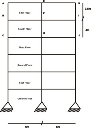
The figures below show the elevation and plan views of a structure. The moments in beams and columns in the fifth storey shall be analyzed. Read on as we take you through a stepwise solution to the problem.
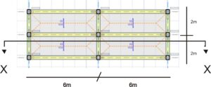
fig1: Fifth floor Plan view showing elevation line XX

fig 2: Elevation view XX
Step 1: The first step to analyzing it is to first draw out the subframe which will include the whole beam span and the adjoining upper and lower floor columns

.
Let us write out the member dimension that makes up the subframe.
Members dimensions
Column AB, DE & GH: Length = 3.5m Cross Section = 300 x 350 mm
Column BC, EF & HI: Length = 4m Cross Section = 300 x 350 mm
Beam BE & EH: Length = 6m Cross Section 300 x 600mm
Slabs: Thickness = 200mm span = 6m x 2m
It should be noted that we have only favored this type of subframe as we want to compute the moment in both beam and columns, other types of subframe can also be used based on the target internal force to be obtained.
Step 2: Compute the slab loads and distribute it on the floor beams
Permanent action
Characteristic Self-weight of slab = 0.2 x 25 = 5KN/m2
super dead Load on Slab = 5.0KN/m2
Characteristic Permanent Load on Slab = 5.0 + 5.0 =10KN/m2
Area of Slab load Supported by Beam 1 = 0.5 x 1 x 2 = 1KN/m2
Characteristic Permanent Load of Slab on Beam = 1.0 x 10 = 10.0KN/m
Self-weight of beam = 0.3 x 0.6 x 25 = 4.5KN/m
Total Permanent Load on beam = 10.0 + 4.5 = 14.5KN/m
Variable action
Variable load on slab = 10KN/m2
Area of Slab load Supported by Beam 1 = 0.5 x 1 x 2.0 =1.0m2
Characteristic Variable Load of Slab on Beam 1 = 1.0 x 10 = 10KN/m
In order to subject the middle column to bending stress, the spans it is supporting shall be asymmetrically loaded. The maximum ultimate load shall be assumed to be acting on a span while the other span is subjected to minimum ultimate load. The maximum and minimum ultimate loads are computed below.
Total Design Load
Maximum ultimate Load acting on Slab =1.35(14.5) + 1.5(10) = 34.6KN/m
Minimum ultimate Load acting on Slab = 1.35(14.5) = 19.6KN/m
We shall convert each uniform load to concentrated load by multiply them by the total length of each beam.
34.6 x 6 = 207.5KN
19.6 x 6 = 117.6KN
Step 3: Assume every support in the beam is fixed and calculate the fixed end moment of the beams. Thus:
$
M_{BE}=\frac{-P\,\,X\,\,L}{8}=\frac{-\text{-207}X\,\,6}{8}=-115.63KNm
$
$
M_{EB}=\frac{P\,\,X\,\,L}{8}=\frac{-\text{207}X\,\,6}{8}=115.63KNm
$
$
M_{EH}=\frac{-P\,\,X\,\,L}{8}=\frac{-\text{-117.6}X\,\,6}{8}=-88.2KNm
$
$
M_{HE}=\frac{P\,\,X\,\,L}{8}=\frac{\text{117.6}X\,\,6}{8}=88.2KNm
$
Step 4 Determine the stiffness of each member
The Stiffness of each member is determined. The columns and the beams have the same cross-section respectively, hence the second moment area of all the columns are the same, and that of all the beams are also equal.
$
For\,\,the\,\,columns,\,\,I\,\,=\,\,\frac{b\,\,x\,\,h^3}{12}\,\,=\,\,\frac{\text{0.3}x\,\,0.35^3}{12}\,\,=\,\,0.001
$
$
For\,\,the\,\,beams,\,\,I\,\,=\,\,\frac{b\,\,x\,\,h^3}{12}\,\,=\,\,\frac{\text{0.3}x\,\,0.6^3}{12}\,\,=\,\,0.005
$
The stiffness of each element member can be calculated using 4EI/L. To make the calculation easier, we can group the members into three according on their length: the upper column, the lower column, and the beams.
The stiffness of each of the upper column is:
$
K\,\,=\,\,\frac{4EI}{L}\,\,=\,\,\frac{\text{4}X\,\,0.001E}{3.5}\,\,=\,\,0.001E
$
The stiffness of each of the lower column is:
$
K\,\,=\,\,\frac{4EI}{L}\,\,=\,\,\frac{\text{4}X\,\,0.001E}{4}\,\,=\,\,0.001E
$
The stiffness of each of the beam is:
$
K\,\,=\,\,\frac{4EI}{L}\,\,=\,\,\frac{\text{4,}X\,\,0.005E}{6}\,\,=\,\,0.004E
$
Step 4 Determine the distribution factor
Since the sub-frame is symmetrical the distribution factor of BA, BC, and BE is equal to that of HG, HI, and HE respectively
$
DF_{BA}\,\,=\,\,DF_{HG}\,\,=\,\,\frac{K_{AB}}{K_{AB}\,\,+\,\,K_{BC}\,\,+\,\,K_{BE}}\,\,=\,\,\frac{0.001E}{0.001E\,\,+\,\,0.001E\,\,+\,\,0.004E\,\,}\,\,=\,\,0.207
$
$
DF_{BC}\,\,=\,\,DF_{HI}\,\,=\,\,\frac{K_{BC}}{K_{AB}\,\,+\,\,K_{BC}\,\,+\,\,K_{BE}}\,\,=\,\,\frac{0.001E}{0.001E\,\,+\,\,0.001E\,\,+\,\,0.004E\,\,}\,\,=\,\,0.182
$
$
DF_{BE}\,\,=\,\,DF_{HE}\,\,=\,\,\frac{K_{BC}}{K_{AB}\,\,+\,\,K_{BC}\,\,+\,\,K_{BE}}\,\,=\,\,\frac{0.004E}{0.001E\,\,+\,\,0.001E\,\,+\,\,0.004E\,\,}\,\,=\,\,0.610
$
$
DF_{ED}\,\,=\,\,\,\,\frac{K_{ED}}{K_{ED}\,\,+\,\,K_{EF}\,\,+\,\,K_{EB}\,\,+K_{EH}\,\,}\,\,=\,\,\frac{0.001E}{0.001E\,\,+\,\,0.001E\,\,+\,\,0.003E\,\,+0.003E\,\,\,\,}\,\,=\,\,0.129
$
$
DF_{EF}\,\,=\,\,\,\,\frac{K_{EF}}{K_{ED}\,\,+\,\,K_{EF}\,\,+\,\,K_{EB}\,\,+K_{EH}\,\,}\,\,=\,\,\frac{0.001E}{0.001E\,\,+\,\,0.001E\,\,+\,\,0.003E\,\,+0.003E\,\,\,\,}\,\,=\,\,0.113
$
$
DF_{EB}\,\,=\,\,\,\,\frac{K_{EB}}{K_{ED}\,\,+\,\,K_{EF}\,\,+\,\,K_{EB}\,\,+K_{EH}\,\,}\,\,=\,\,\frac{0.003E}{0.001E\,\,+\,\,0.001E\,\,+\,\,0.003E\,\,+0.003E\,\,\,\,}\,\,=\,\,0.379
$
DFEB = DFEH = 0.379
NB: You may notice that some of the value of the distribution factors differ in spite that there are corresponding figures representing stiffness at the numerator and denominator respectively (E.g: DFBA vs DFBC). This happens because the actual values use in the calculations are not the approximated values displayed in this solution. The un-approximated figures are used hence the little differences. This explanation also applies to the earlier computation of stiffness.
In order to make our iteration concise and tidy when making the moment distribution operations, it is a good practice to group columns meeting at a joint together. To implement this, we add together the distribution factors of column meeting at a joint so that the columns can be treated as a single member.
DFAB + DFBC = 0.207 + 0.182 = 0.389
DFED + DFEF = 0.129 + 0.113 = 0.242
DFHG + DFHI = 0.182 + 0.610 = 0.390
Step 5: Enter the values of the fixed end moment and distribution factor in a table and initiate subsequent iterations.
The values of fixed end moment and Distribution factors will be entered in a table as shown below

The next thing is to calculate the out of Balance Moment (OBM), and then the carry-over moment like that of any other moment-distribution operation until the moments at the supports reasonably converges. If the operations are diligently carried out, the result should be as that as shown below:
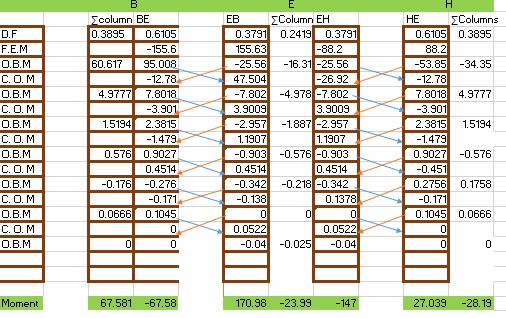
The moment at each beam end can be extracted directly from the table. BE = -67.58KNm, EB = 170.98KNm, EH = -147KNm, and HE = 27.039KNm
The moment of individual column at a joint can be gotten by multiplying the overall moment of the columns meeting at that particular joint by the distribution factor of each of the column in turn. This is carried out below:
$
M_{BA}\,\,=\,\,\text{67.581,}X\,\,\frac{K_{BA}}{K_{BA}\,\,+\,\,K_{BC}}\,\,=\,\,\text{67.581,}X\,\,\frac{0.001}{\text{0.001}+\,\,0.001}\,\,=\,\,36.0KNm
$
$
M_{BC}\,\,=\,\,\text{67.581}X\,\,\frac{K_{BC}}{K_{BA}\,\,+\,\,K_{BC}}\,\,=\,\,\text{67.581}X\,\,\frac{0.001}{\text{0.001}+\,\,0.001}\,\,=\,\,31.5KNm
$
$
M_{ED}\,\,=\,\,\text{23.991}X\,\,\frac{K_{ED}}{K_{EF}\,\,+\,\,K_{ED}}\,\,=\,\,\text{23.991}X\,\,\frac{0.001}{\text{0.001}+\,\,0.001}\,\,=\,\,12.8KNm
$
$
M_{EF}\,\,=\,\,\text{23.991}X\,\,\frac{K_{EF}}{K_{EF}\,\,+\,\,K_{ED}}\,\,=\,\,\text{23.991}X\,\,\frac{0.001}{\text{0.001}+\,\,0.001}\,\,=\,\,11.2KNm
$
$
M_{HG}\,\,=\,\,\text{28.191}X\,\,\frac{K_{HG}}{K_{HG}\,\,+\,\,K_{HI}}\,\,=\,\,\text{28.191}X\,\,\frac{0.001}{\text{0.001}+\,\,0.001}\,\,=\,\,15.035KNm
$
$
M_{HI}\,\,=\,\,\text{28.191}X\,\,\frac{K_{HI}}{K_{HG}\,\,+\,\,K_{HI}}\,\,=\,\,\text{28.191}X\,\,\frac{0.001}{\text{0.001}+\,\,0.001}\,\,=\,\,13.156KNm
$
It is worthwhile to call your attention again to the fact that in spite that the figures in both the numerator and denominator of the distribution factor relating to one or two columns corresponds with one another, the final moments distributed to them still differ. This is because the figures used in the actual computations are un-approximated unlike those displayed in the actual calculations above.

good work